Quick Fourier Series Intro

url: https://www.youtube.com/watch?v=mgXSevZmjPc
title: The Fourier Series and Fourier Transform Demystified
channel: Up and Atom
duration: 14m 47s
visited: 2023-06-27

The Fourier Series, and the Fourier Transform, can be found almost everywhere. The concept is that we can kind of write almost any function in terms of sine and cosine. But how so? They have a very smooth shape, but things like a square-wave or saw tooth wave have jagged edges.

We need to start at the beginning.

Adding Functions Together

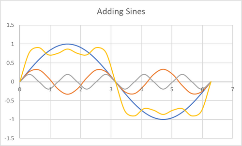
Markdown makes photos challenging… but imagine a regular sine wave, $\sin(x)$ on the interval $[0,2\pi]$. Now, imagine $\sin(3x)$ on that same interval. It has a smaller frequency. If you add them together, you may see how we begin to approach a new graph. That is, over the same $x$ interval, we add together the $y$ values of the function.

In that example, you’ll also notice that when the results in the original functions are both the same, the sum gets larger (either positive or negative). And when the signs are opposite, they cancel each other out.

Since our example above has moments that cancel each other out, we want to give our $\sin(3x)$ a smaller amplitude, to hinder the effect it has. If we continue to add similar terms, smaller amplitude and frequencies, you’ll see it approaches the square wave.

Above is a small graph made in Excel. The sine waves are different frequency and amplitudes of the sine function and the Yellow is the addition of them. As we continue to add more waves, we’ll get closer to the square wave.

The Fourier Series is an infinite sum, meaning you’ll add infinite waves. Therefore, you’ll eventually reach your exact solution.

Another example is the saw tooth wave. You can start with the following:

What is the point, especially when it involves an infinite sum? In practice, we don’t need to evaluate an infinite sum, but just enough terms to be good enough for the application. The instructor suggests a program to determine the difference between our two functions, the square and sawtooth waves.

Just by knowing the amplitude (coefficient) of the second term, the program could tell the difference.

Finding the Fourier series for a trivial example like this might be more work than it’s worth. However, extending this to different and more general objects helps a computer learn pattern and shape recognition. The difficult part, when comparing objects, is finding the Fourier Series to analyse. That is, what waves make up the shape we are looking at.

The Fourier Transform help determine which waves make up the Fourier Series. It can also pick and remove waves without having to find the Fourier series as well. This help when removing noises in recordings.

The idea is that you give it amplitude vs time function, and you get an amplitude vs frequency function. This happens because the transform decomposes the function into sine and cosine waves. The graph of AvF looks like a bar chart. It is a “frequency domain view of a time domain function.”

Mathematical equation for Fourier transform $F(\omega)$ is

The $f(x)$ is the time function we are calculating the Fourier Series for. The exponential term comes from Eulers Formula…

Basically, you can write the exponential in terms of sine and cosine waves. Also, that $i$ is for an imaginary component. It handles the general case where there may be different phases required to make up the function.

For the square wave, it ends up looking like $F(3) = \int f(x) [\sin(3x)] dx$. We multiple values from the sine wave and our function to get some results, either positive or negative. When the results are positive, it tells us the results are more correlated. And when the waves are anti-correlated, we will get a negative value. And when there is no correlations, we get 0. In this, the terminology for correlation more or less means the difference between actual and expected, more like a variance, but not.

The integral is a continuous version of the sum. We are summing all of the correlations to determine if the wave is important to the series. If the term is important, its sum will be greater than 0. If the sum is negative, it’s not useless, but just subtracted instead of added because it implies anti-correlation.

For the square wave, the integral of our $\sin(3x)$, and after normalization, we find the sum to be $\frac{1}{3}$. This means that one-third of the amplitude is used to make the square wave! really cool.

The square wave is only made up of odd sine curves. That is because, there’s one extra ‘hump’ in each odd term to make the resulting summation not 0. Similar reason why the cosine value isn’t seen in this series either.

The Fourier Transform does this process for any frequency, telling us which frequencies go into any function. You can think of it as “Changing the basis of the function in an infinite dimensional space.” What does this mean? We can change the basis of function space, like how we change the basis of a vector space, which is change coordinates to describe the same vector. So, we went from amplitude vs infinite time positions, to amplitude vs infinite frequency values. This is only possible because our sine and cosine waves make up an orthogonal basis. Or, they can be combine to make any function in function space.

The catch is that you need some kind of mathematical description of the input function. This is where algorithms come into play. Plug in for Curiosity Stream. Additional plugin for Nebula.TV.

Applied Fourier Analysis

title: Applied Fourier Analysis
subtitle: From Signal Processing to Medical Imaging
author: Tim Olson
publisher: Springer Science+Business Media, LLC
year: 2017
doi: https://doi.org/10.1007/978-1-4939-7393-4_1

1. Introduction: From Linear Algebra to Linear Analysis

Fourier Analysis is at the center of many modern sciences, from Physics and engineering, to population dynamics in biology. Many of the important phenomena in our world are related to periodic phenomena. Understanding frequency based functions, sines and cosines, are eigenfunctions, or “building blocks of the universe.”

1.1 Three variations of Fourier Analysis

1. Fourier Series
2. The Discrete Fourier Transform
3. The Continuous Fourier Transform

Fourier Series involves representing a continuous function on a finite interval $[a,b]$ with an infinite series, which is similar to the Taylor series.

The Discrete Fourier Transform (DFT) is focused on a function on a finite set of points, referred to as $0,1,\text{...},N-1$. Being discrete, it’s commonly implemented in technology.

The Continuous Fourier Transform (CFT) extends the Fourier Series to deepen our understanding of connections between physical reality and digital representations.

1.1.1 Fourier Series

Quick look at a basic Fourier Series. On an interval $[-\pi, \pi]$ we can represent a series expansion:

where…

Ok, so that is a discrete summation of the integration of trigonometric functions on our interval for each value of $k$. We have only just begun the most basic form of Fourier Analysis, which is to separate a function into the various frequencies which represent it.

Interesting to note that the cosine terms are even, and the sine terms are odd. We have decomposed our function into even and odd parts, in addition to individual frequencies. This will be invaluable later.

One limitation of the Fourier Series can be seen in the formulas. You must calculate the integrals, a time consuming and difficult practice. Another limitation is that a Fourier Series is only valid on a finite interval.

1.1.2 The Discrete Fourier Transform

The Discrete Fourier Transform (DFT) addresses the problem of calculating an infinite number of integrals by creating a simple matrix that can be on basic finite signals.

Suppose you have a function $f(t)$ on an interval, and you need to represent with $N$ samples at discrete time points $t_n$, where $n=0...N-1$. We will let this be a vector:

formula 1.1

The DFT samples cosine and sine terms. The vector representing $cos(t)$ would be $\cos(\frac{2 \pi n}{N})$, where of course $n=0, 1,\;...\;,N-1$. Both will go through a complete cycle on the interval of $[0, 2\pi]$.

We use the sine and cosine vectors to construct the Fourier Matrix $F_N$, where $N$ represents the number of points in our sampled function. We can write the vector as a multiple of these cosine and sine vectors:

equation 1.2

We let $c$ represent the coefficients of our sampled sines and cosines. Note, you can easily find $\vec{c}$ if needed. Advantages:

• No integral calculations
• Can decompose matrix $F_N$ in a special way to make Linear Algebra Fast.

We must address several issues / questions to utilise this approach:

1. How often to sample to be accurate? How small do time intervals need to be?
2. Do we utilise the matrix on short portions of function, or long portions?
3. Will this represent the real frequency content of the original function?
4. Can we calculate these expansions quick enough to be useful in applications such as real-time communication systems?

1.1.3 The Continuous Fourier Transform

We define the the Fourier Transform as:

The final integral is composed of sine and cosine subsets. These discrete subsets, or samples, of the Fourier Transform generate sampling theory, which we will also look at later.

We use the Continuous Fourier Transform to more easily understand some beautiful phenomena. One such being the uncertainty principle.

1.2 Motivations

1.2.1 Exploration and Understanding

A primary goal of science is to provide simple explanations of a phenomenon. A lot of physical phenomena can be explained with sines and cosines.

One such example is the begins with an ordinary differential equation:

One way to solve the equation is to guess the solution takes the form of $y=e^{\lambda t}$. That easily leads to the derivatives. Then there is some older, weird logic like this:

But since $e^{\lambda t} \neq 0$ for any $t$, we just factor it out…

The solution then depends on the above equations, a typical polynomial. We have changed a differential equation into a simple polynomial equation. Then, we can solve with the quadratic equation:

quadratic equation

If the discriminant, $(b^2-4ac) >0$, then the solutions are both real and the corresponding solutions to the differential equation will exhibit either exponential growth or decay.

For reference, exponential growth is typical of population growth, like bacteria in a petri dish. An exponential decay is common in situations where a signal is being absorbed as it transmits through a medium. I think calculations of half-life exhibit exponential decay.

Prep for the next topic; conjugates are pairs of binomials with identical terms but parting opposite arithmetic operators in the middle. An example being $(3-2i)$ and $(3+2i)$.

Fourier Analysis is useful for when $b^2-4ac < 0$. The $\lambda$’s with be conjugate pairs of one another, which can be denoted as $\lambda_{\pm} = \alpha \pm i \beta$.

Also note that $i = \sqrt{-1} \; \therefore \; i^2=-1$. Hence, a complex exponential solution(s):

It is generally assumed that $\alpha \leq 0$. If $\alpha = 0$ the solution would oscillate forever. However, when $\alpha < 0$, the solution to the differential equation decays exponentially to zero.

The frequency $\beta$ is often called the resonant frequency of the system.

1.2.2 Manipulation

We might want to manipulate output or behaviour of a system:

• remove background noise or static from audio
• Emphasize major long-term trends in a system
  • They can be clouded by a number of minor and less important short-term phenomena
• Clearly enhance radar signals for air traffic controllers

1.2.3 Compression

Simple changes to the way things are represented and stored can save vast amounts of storage space. Compression information without losing quality, transmission, and restoration of information is very valuable, especially in communications.

1.2.4 Practice

Using Taylor Series expansion of $e^x$, show that

To do this, you will need this list of Maclaurin series of common functions. Colin Maclaurin, in the mid-18th century, created this list of when $0$ is the point where the derivatives are considered.

Let’s write down what we are looking for

Looking at the middle pattern, It’s really interesting that the combination covers all values of $x$.

Additionally, the Riemann Series Theorem, named after 19th-century German mathematician Bernhard Riemann, states that if an infinite series of real numbers is conditionally convergent, that it does not converge absolutely, the terms can be arranged in a permutation so that the new series converges to an arbitrary real number… or diverges. This implies that a series or real numbers is Absolutely Convergent if and only if it is Unconditionally Convergent.

• Unconditionally convergent = all reorderings of a series converge to the same value.
• Conditionally convergent = series can converge to different values based on ordering.
• Absolute convergent = sum of all absolute values of summands is finite.

The series are meant to be absolutely convergent, meaning they can be rearranged without affecting the outcome.

And finally:

Either way:

Now, let’s do a little calculus comparison

We know that

Therefore

Now,

Based on the Maclaurin series for cosine and sine, I’m not getting similar results, but didn’t try too hard as I am pressed on time.

Additionally, try to differentiate $e^{\alpha t + i \beta t}$ and $e^{\alpha t}(\cos(\beta t) + i \sin(\beta t))$. Do they line up better?

1.3 Linear Algebra, Linear Analysis, and Fourier Analysis.

Fourier Analysis is an extension of Linear Algebra. It is the study of sines and cosines, and how they interact and behave in a complex setting. Fourier Analysis is a subtopic of Linear Analysis, which is an extension of Linear Algebra, following the same rules, except that we allow an infinite number of variables, or dimensions.

Basic concepts of Linear Analysis are the same as Linear Algebra. Begin with the idea of a vector space, which involves objects and operations.

2 types of objects:

• Scalars $\to$ Usually real or complex numbers.
  • We insist scalars come from a field meaning they behave like real or complex numbers.
• Vectors $\to$ Ordinary vectors in Linear Algebra.
  • These will often be sines and cosines in Fourier Analysis

2 types of operations:

• Scalar multiplication
• Vector addition

We now have the basics in a vector space. Consider that we are $R^n$, and we have a matrix. According to Linear Algebra, if we have a matrix $A$ within a vector space, it holds that

That is, the matrix respects the linear arithmetic of the vector space.

1.3.1 The Dot Product, Inner Product, and Orthogonality

The dot product is used extensively in Linear Algebra, and defined as:

definition of dot-product

It has many implications, one being it defines the notion of distance:

notion of distance

This can be seen as an extension of the Pythagorean theorem. Sum of the squares equals the final vector squared. We define length as:

We can also measure angles between vectors:

The above is the for an angle between any two vectors in $\mathbb{R}^3$.

Additionally, these equations provide fundamental inequalities. Since $|\cos(\theta)| \leq 1$, the Cauchy-Schwartz inequality follows,

Note that it is hard to visualise angles between $\mathbb{R}^n$. However, We measure the angle on the subspace created by the 2 vectors. In $\mathbb{R}^n$, any two vectors define a two-dimensional subplane, and therefore the angle is also well defined.

We will move now to the Inner Product, which will be defined after a quick discussion. Consider a function on an arbitrary interval $[a,b]$. We want to measure the length and angle between any two functions. We will consider functions $f(t)$ and $g(t)$. Now, the vectors:

With $N$ points, we have approximations to the functions in $\mathbb{R}^N$. Take their dot product:

An issues is this dot product is arbitrary depending on how we pick points $t_k$. If the points are close together, perhaps we could derive a useful meaning about the functions. But including twice as many points will make the result nearly twice a big. Therefore, we include a factor for the distance between points:

The above is actually a Riemann Sum. And thus, why not let that distance approach $0$?

Definition 1.3.1 - The Inner Product: if $f(t)$ and $g(t)$ are two functions on an interval $[a,b]$, we define their inner product to be:

definition of inner product

As long as the Riemann sum converges, it converges to the inner product.

Operations:

• Computation
  • Dot Product $\to$ $\vec{a} \cdot \vec{b} = \sum a_kb_k$
  • Inner Product $\to$ $\langle f(t), g(t) \rangle = \int_a^b f(t)g(t)\,dt$
• Length
  • Dot Product $\to$ $|\vec{a}|^2 = \sum |a_k|^2 = \vec{a} \cdot \vec{a}$
  • Inner Product $\to$ $\|f(t)\|^2 = \langle f(t),\, f(t) \rangle = \int |f(t)|^2 \, dt$
• Angle
  • Dot Product $\to$ $\vec{a} \cdot \vec{b} = |\vec{a}||\vec{b}| \cos(\theta)$
  • Inner Product $\to$ $\langle f(t),\, g(t) \rangle = \|f(t)\| \| g(t) \| \cos(\theta)$
• Inequality
  • Dot Product $\to$ $|\vec{a}\cdot\vec{b}| \leq |a||b|$
  • Inner Product $\to$ $\langle f(t),\, g(t) \rangle \leq \|f(t)\| \| g(t) \|$

Moving onto Orthogonality! p. 12 Perpendicular, orthogonal, right angle, they imply the same thing in our context. Although, I believe perpendicular is more geared towards a plane in 3D space.

Fun identity, 2 vectors are orthogonal if their dot products, or inner products, are 0. This also happens with $\cos(\theta) = 0$ assuming the functions themselves are nonzero.

A set of functions is orthogonal if the dot product or inner product of every subset of two of them is 0. That can be a lot of math.

Collections of vectors or functions are orthonormal if they are orthogonal, and each has length 1, like a unit vector.

1.3.2 Eigenvectors and Eignevalues in Linear Algebra

It is assumed the reader is familiar with Linear Algebra.

I will hopefully, one day, include a complete linear algebra section! Until then, I suppose having a quick recap can’t hurt anything besides my fingers from all of this typing…

We will cover the concepts of Eigenvectors $\vec{v}$ and corresponding Eigenvalues $\lambda$, as the title suggests. For a square $n \times n$ matrix $A$:

Where $\lambda$ is some scalar, and the pair together is called an eigenpair. Should be obvious that the direction is consistent, but the magnitude has changed. Even if $\lambda < 0$, the vector points in the opposite direction but is still parallel.

A mention of common principles from Linear Algebra:

• Linear independence = A collection of vectors is said to be linearly independent if non of the individual vectors can be represented by a sum of the other vectors.

The author says that a Linear Algebra book will cover these important topics, so I’ll defer to that.

Then there is the fundamental idea of diagonalization. Suppose we have a matrix $A$ that has $n$ linearly independent eigenvectors $\vec{v}_j$, with corresponding eigenvalues $\lambda_j$, assuming all are real for now. For any $n$-dimensional vector $\vec{x}$, we write:

equation 1.4

We then want to multiply matrix A by $\vec{x}$. Using linearity…

equation 1.5

However, if we know the eigenvalue, we can use that instead.

This is better for many reasons:

• Reducing matrix multiplication into scalar vector multiplication.
• Using $n$ individual eigenvectors instead of an arbitrary large matrix. It makes interpretation easier.
• We have reduced a potentially large confusing matrix into a bunch of one-dimensional eigenvector problems.

1.3.3 Orthogonal Diagonalization

An additional restriction to diagonalization we must consider is that matrix $A$ must also have orthogonal eigenvectors. We mean the dot product:

Then, store these eigenvectors as columns of matrix $V$ and normalize the entries of $V$ that have length one, so $\vec{v}_i^t \vec{v}_i = 1$. We now have

You can then write that:

Apply $A$ to $x$ to get the following:

Now, lets take it one piece at a time…

To simplify

Matrix multiplication has been reduces to a series of dot products with eigenvectors, multiplied by eigenvalues. This is sometimes called the EigenFunction approach.

1.3.4 Diagonalization in Linear Analysis: Eigenfunctions

p.14

Let’s start with eigenfunctions. In linear analysis, eigenfunctions are a special type of function that have a unique property when operated on by a linear operator. A linear operator is a mathematical operation that takes a function as input and produces another function as output.

When an eigenfunction is operated on by a linear operator, the resulting function is a scaled version of the original eigenfunction. In other words, the output is the same shape as the input, but it may be stretched or compressed by a certain factor. This scaling factor is called the eigenvalue.

To give you an analogy, think of a rubber band. If you stretch or compress the rubber band, it changes in size, but it retains its original shape. Similarly, an eigenfunction behaves like a rubber band under the action of a linear operator.

Now, let’s move on to diagonalization. Diagonalization is a process in linear analysis that allows us to simplify the representation of a linear operator. The goal is to find a special set of eigenfunctions that make the operator’s behavior easier to understand and work with.

When a linear operator is diagonalized, it means that its representation can be written as a diagonal matrix. A diagonal matrix is a square matrix where all the elements outside the main diagonal (from the top-left to the bottom-right) are zero. The values along the main diagonal correspond to the eigenvalues of the operator.

Diagonalization is useful because diagonal matrices have simpler properties compared to general matrices. Operations such as multiplication and exponentiation are much easier to perform on diagonal matrices.

To illustrate diagonalization, imagine you have a box of differently sized rubber bands (representing eigenfunctions) and a stretching machine (representing the linear operator). You put the rubber bands into the machine, and out comes a collection of rubber bands, each stretched or compressed by a certain factor. If you arrange these rubber bands according to their stretch factors, you end up with a diagonal configuration where each rubber band represents an eigenfunction, and the stretch factor represents the eigenvalue.

By diagonalizing a linear operator, we gain insights into its behavior and can perform calculations more efficiently.

Consider the following:

Letting $t=0$ will eliminate the cosine factor and also give us the initial displacement of the system. Notice that the frequency of the time variation, the cosine factor, is tied to the frequency of the spatial variation, the sine factor. This is the fundamental nature of the wave equation, discussed in at a later time.

1.3.5 Fourier Analysis

Fourier Analysis is involved in many studies that are centred around waves, like study of light and optics, sound, etc… When you learn Fourier Analysis, you position yourself to better understand that entire list of topics.

1.3.6 Notational Differences

We will typically refer to the Fourier Transform of a function as:

An author, Rob Bracewell, of another esteemed book, refers to the following:

Ch. 2 Basic Fourier Series

This is a quick introduction into the basics where the reader can then dive further into interesting topics on their own.

2.1 Fourier Series on $L^2[a,b]$

Definition 2.1.1 The set of functions $f(t): [a,b] \to R$ whose squared integral is finite, i.e. $\int_a^b|f(t)|^2 \lt \infty$ is referred to as $L^2[a,b]$, the square integrable functions on $[a,b]$.

The square integrable functions for the space of functions that we are interested in. Also consider:

call it equation 2.1

The first 2 integrals are finite because $f(t),\,g(t) \in\; L^2[a,\,b]$. The last integral is finite because of Cauchy-Schwartz Theorem:

Therefore we can say it is a vector space. Of course, the proof of when the functions are complex would be left as an exercise because why sell a book that actually explains everything?

Theorem 2.1.1 Let $f(t)$ be any function in $L^2[-\pi, \pi]$. Then, we can represent $f(t)$ in a series as

Where

This means you can represent any function in $L^2[-\pi, \pi]$ as the sum of sines and cosines.

Theorem 2.1.2 Let f(t) be any function in $L^2[a,b]$. We can represent $f(t)$ in a series as:

Where

Additionally

Theorem 2.1.2 is just a generalisation of 2.1.1.

We can now simplify the theorem if the interval is centered about the origin, $a = -T$ and $b = T$.

Corollary 2.1.3 Let $f(t)$ be any function in $L^2[-T,\,T]$. Then, we can represent $f(t)$ in a series as:

Where

The author then explains how to get from theorem 2.1.1 to 2.1.2 in case you have trouble memorizing, or looking them up.

2.1.1 Calculating a Fourier Series

The issue is that we have to calculate an infinite number of integrals. You can actually calculate them simultaneously. However, the Fourier Series cannot typically be easily calculated by hand.

As an example, consider the characteristic function on $[-\pi,\,\pi]$ to be:

Other ways you may see this function are…

or

We would like to start by calculating our coefficients.

Definition 2.1.2 - Even and Odd Functions: A function $f(t)$ is said to be even if $f(t) = f(-t)$. And it is odd if $f(t)=-f(-t)$.

This matters because cosine is even and sine is odd. If $f(t)$ is odd, then $\int_{-T}^{T}f(t)dt=0$. Additionally, the products of these functions corresponds to positive and negatives. So, if $f(t)$ is even, then $f(t) \sin(kt)$ is odd, and $b_k$ terms will zero out. The logic being that even functions can be represented entirely by cosine terms. Opposite logic applies if $f(t)$ is odd.

We note that $\chi(t)$ is even.

We now solve for terms in 2 parts, which is a plug and chug scenario based on substituting values in from our characteristic function. The author uses the odd property of sine that $\sin(x) - \sin(-x) = 2 \sin(x)$.

The author continues to arrive at

Remember, this is a transformation. So, it still represents the original function, just in a different context. But an infinite sum isn’t really programmable. As $k$ get bigger, the denominator grows, and therefore the result continues to decrease. We can probably take a partial sum as a good approximation, written as follows:

How many terms makes a good approximation? Might be useful to look at an error metric.

The next example would be the super simple function $f(t) = t$ on the interval from $[-\pi, \pi]$. Off the bat, note that this is an odd function, so it will be exclusively defined through sine. Then, calculate the coefficient using integration-by-parts.

You can probably tell that more complex functions get out of hand. We will look into other methods of calculating the coefficients, probably numerical approximations.

2.1.2 Periodicity and Equality

Fourier Series can approximate nearly any function over a finite interval. Don’t make the mistake of believing that the FS will represent anything outside an interval though. Coefficients were determined and depend on $f(t)$ in that interval.

Also, $f(t)$ doesn’t necessarily need to be periodic at all. Thus, again, we can’t expect $S_{[a,b]}(f)(t)$ to represent $f(t)$ outside of the defined interval. We may also use the notation $S_{\pi}(f)(t)$ to denota the Fourier Series on $[-\pi, \pi]$.

We are now looking into the function of the Four Series.

The right is an infinite sum. We want to say the limit as the number of terms approaches infinity converges to $f(t)$, but that’s apparently not correct.

We define:

and the error function is:

As the limit of our $n$ terms approachs infinity, the error will approach 0 for any function $f(t) \in L^2[a,b]$. Beyond our scope, research books that discuss the relative convergence rates of Fourier Series.

2.1.3 Exercises

Compute the Fourier Series for the function:

on $[-\pi, \pi]$. Plot some terms both in and outside the interval.

Try to compute it now on a larger interval, like $[-2\pi, 2\pi]$.

Try $f(t)=t$ and $f(t)=t^2$ on similar intervals. It’s mostly finding sine and cosine coefficients.

2.2 Orthogonality and Hilbert Spaces

Orthogonality and perpendicularity are the same concepts, used interchangeably. However, we typically say orthogonal when dealing with dimensional vector spaces greater than 3 dimensions, or the function spaces, like $L^2[a,b]$.

Dot product: defined here

Euclidean distance: $|\vec{a}| = \sqrt{\vec{a} \cdot \vec{a}}$

Angle between vectors: $\vec{a} \cdot \vec{b} = |a||b| \cos(\theta)$.

We now want to compare two functions $f(t)$ and $g(t)$. Consider finite number of points $t_k$, where $t_0=a$ and $t_n=b$ on the interval $[a,b]$.

Distance between each point is defined as $\delta t = (b-a)/n$.

We want to approximate the length of these functions by their vector counterparts.

However, if we have more points, then the length could double. So, we then multiply in

Thus, on the same interval, if we cut it put into more pieces, each piece has a smaller weight.

Definition 2.2.1 - Inner Product: if $f(t)$ and $g(t)$ are functions in $L^2[a,b]$, then we define the inner product as:

And the length of $f(t)$ would be

We used complex conjugate in the inner product definition, which is a number with equal real and imaginary parts, equal in magnitude but opposite in their sign.

Standard Linear Algebra, or linear analysis, texts should dive into details about the inner product.

Stating the important properties inhertied by $L^2[a,b]$:

• Linearity - if $f$ and $g$ are functions in an inner product space, then so is $c_1f+c_2g$.
• if $f \neq 0$, then $\|f\| \neq 0$.
• Triangle rule - if $f$ and $g$ are in an inner product space $\|f+g\| \leq \|f\|+\|g\|$.
• Cauchy-Schwartz Inequality - If $f$ and $g$ are inner product space

The equality holds only if $f$ is a constant multiple of $g$, $f(t) = cg(t)$.

Definition 2.2.2.a Two functions $f(t)$ and $g(t)$ in $L^2[a,b]$ are said to be orthogonal if $\langle f,g \rangle = 0$. A collection or set of functions $\{ o_k(t) \}_{k=0}^N$ is orthogonal if for any pair of functions from the set $\langle o_i,o_j \rangle = 0$ where $i \neq j$.

Definition 2.2.2.b We say that a set of functions is orthonormal if they are orthogonal, and they all have length one, $\|o_j\| = 1$.

Theorem 2.2.1 - Orthogonality: The functions $\{ \cos(kt) \}_{k=0}^{\infty}$ and $\{ \sin(kt) \}_{k=0}^{\infty}$ are orthogonal on the interval $[-\pi, \pi]$. Additionally, functions used in Theorem 2.1.2 are also orthogonal on corresponding interval $[a,b]$.

Proofs on pp. 32-33

Because of odd and even trig functions

Thus, cosines are orthogonal to all sines.

Interesting as well, given double angle trigonometric identities…

The proof goes on to prove cosines are cosines are orthogonal to each other and similar logic for sines orthogonal to each other as well.

2.2.1 Orthogonal Expansions

Completeness refers to having enough functions for the expansions we are suggesting. It’s beyond the scope of the text. The author provides a proof of completeness pp. 33-34.

Theorem 2.2.2 Let $\{o_k\}$ be a complete set of orthonormal functions in $L^2[a,b]$ then for any function in that space:

2.3 The Pythagorean Theorem

It’s fundamental to Fourier Analysis. Note that a vector space is a set of elements, called vectors, that can be added together and multiplied by scalars. The Hilbert space is a vector space where the inner product also lives as a distances function.

Further, but not necessary, a Euclidean space are intended to represent physical space.

Theorem 2.3.1 - Pythagorean Theorem: let $f(t)$ be a function in a Hilbert space $H$, like $L^2[a,b]$. Let $\{ o_k \}_k$ be a complete set of orthonormal functions and $f(t)$ be an element of $H$. The squared length of $f$ can be represented as:

There’s a proof on p.36

… skipping ahead to convolution for time sake…

2.8 Convolution and Correlation

Definition 2.8.1 - Convolution and Correlation: Let $f,g \in L^2[-T,T]$, and by extensions $L^2[-2*T,2*T]$. The convolution of $f$ and $g$ is:

And the correlation of $f$ and $g$ is:

Subtle difference in the function $g$. We want to characterize the Fourier Series of these two function. I think it’s basically taking 2 functions and making a third function.

Theorem 2.8.1 - Convolution and Correlation Theorem: Let $f,g \in L^2[-T,T]$. the convolution $f*g$ will be in $L^2[-2T,2T]$. Further, the Fourier Series of $f*g$ on $L^2[-T,T]$, denoted $\mathcal{F}(f*g)$, expressed as:

The Fourier Series of correlation is:

$\mathcal{F}(f)$ maps the function $f$ to its Fourier Coefficients.

Proof found on p. 66.

We continue to skip Chapter 3 which is the Discrete Fourier Transform

Ch. 4 The Fourier Transform

We relax the assumption that $L = 2 \pi$, the Fourier series is:

You can write the frequency as $\omega_n = 2 \pi n/L$ to rewrite the above equation.

We also previously too the period $L$ to be a finite interval after which the function repeats itself. But we can also consider the limit of large periods, $L \to \infty$. What would happen is that the difference in frequencies in sine and cosine terms becomes infinitesimally small and they become a continuum.

Recall coefficients are given by:

Substitute this expression into the complex Fourier Series,

It looks complicated, but if we let $L \to \infty$, then $\Delta \omega \to 0$. This simplifies to:

We apparently chose $x_0 = -L/2$. Put it together: