title: Hands-On Machine Learning with Scikit-Learn, Keras, and TensorFlow
subtitle: Concepts, Tools, and Techniques to Build Intelligen Systems
edition: 3
authors:
	- Aurélien Géron
publisher: "O'Reilly Media, Inc."
date: Oct. 2022
This is a large book, over 800 pages, and the last for my Data Science course. If you are interested in reading yourself, you can get a nice pdf from eBooks.com. I would love to do an extensive deep dive into this book, especially the Reinforcement Learning section, but I don’t think it’s possible right now.
In 2006, Geoffry Hinton et al. published a paper, “A Fast Learning Algorithm for Deep Belief Nets”, regarding how to train a deep neural network. Others previously gave up on the idea, but this was the start of the tech-splosion we are seeing today.
Naturally, we want to also build cool technology. Luckily, this book assumes little-to-no previous knowledge of machine learning. It relies on Python frameworks:
Scikit-Learn - Great entry point for learning ML.TensorFlow - More complex library for distributed numerical computation.Keras - a high-level DL API, comes bundled with TF.You should be familiar with Python and scientific libraries such as Numpy, Pandas, and Matplotlib. You should also be familiar with linear algebra.
This is the high-level overview chapter.
Machine learning is the science and art of programming computer so they can learn from data. It is the field of study to give computers the ability to learn without being explicitly programmed.
A system learns from a training set. A model is the part of the ML system that does the learning. There’s training data too. One performance measurement is accuracy.
For the example of a spam filter, coding explicitly would generate a very long list of complex rule that becomes hard to maintain. A machine learning program can learn the rules based on data and sort emails in a much more efficient and maintainable way. Digging into data to discover hidden patters is called data mining.
There are a lot of different systems, so we can give a little criteria here:
The book goes over these in greater detail.
Transfer learning occurs when knowledge from one task is transferred to another. It is one of the most most important techniques in machine learning today, especially in deep neural networks.
Reinforcement learning is very different from what we have previously discussed. It has a learning system that we call an agent. It observes the environment, selects and performs actions, and receives rewards in return, or penalties. It learns on its own what the best strategy is, called a policy, to get the most reward over time.
The book also throws in an example of using Scikit-Learn for a quick linear regression model (p. 25). It is really cool how easy it is.
p. 27
The main tasks are selecting a model and training it with data. That means two sources or error:
Even simple problems solved with ML require thousands of examples. More complex problems like image and speech recognition might need millions. There have been papers, like one titled “The Unreasonable Effectiveness of Data” that discusses how data can be just as important, or even more so, than the algorithms.
For either instance-based or model-based learning, it is crucial that the training data be representative of new cases you want to generalize to.
If your data set is too small you can have sampling noise, which is like nonrepresentative data as a result of chance. And if sampling method is flawed for even large methods, they can be nonrepresentative, something referred to as sampling bias.
Nonresponse bias is a type of sampling bias that occurs in a survey when a majority of people done respond.
There’s another section on Data Quality, it’s basically its own course. The majority of time spent in a data science project is on cleaning data.
“Garbage in, garbage out!” A data scientist needs to have the correct set of features to train on. This is called feature engineering, which involves the following:
p. 30
Overfitting happens when a model performs well on training data but cannot generalize well when tested against other data.
I like to think of it as studying for a math test. The computer first tries to learn patterns in questions and answers. However, if training too long, it begins memorizing answers to questions. That won’t extend well to questions not in the training set.
Additionally, if your data is noisy, the model may learn patterns in the noise itself. Also, if data is not great, the model could detect chance coincidences and remember them as policies.
Overfitting happens when the model is too complex relative to the amount and noisiness of training data. Some possible solutions are:
Constraining the model to make it simpler is called regularization. The amount of regularization to apply during learning can be controlled by a hyperparameter, which is a parameter of the learning algorithm and not the model.
Underfitting is the opposite of overfitting, and occurs when the model is too simple to learn patterns in the data provided. It you get poor results from a simple model, like a linear model, you could try the following:
Typically, before deploying in production, you test the model. Basically, split your data into training and testing sets. The error rate on the test set is the generalization error. If the training error is low, but testing is high, that’s a sure sign of overfitting.
Suppose we train a linear model and apply regularization to avoid overfitting. We choose the right hyperparameter by training 100 different models with same number of different hyper parameters. I think this is like cross-validation in scikit-learn or something.
So, you get the right hyperparameter(s), only 5% error, deploy the model and… 15% error, what?!? Well, we measured the generalization error multiple times and found hyperparameters for that particular set.
A common solution is having a holdout validation set, which is part of the training set to select the best candidate model. This has many name, validation set, development set… that’s it actually.
So, it is really a training set, testing set, and validation set.
Yes, so you can perform repeated cross-validation with many small validation sets to more accurately a models performance. This requires a lot of training
It might be easy to get a lot of data but that doesn’t mean it will perfectly represent data used in production. Important to remember that both the validation set and test set must be as representative as possible of data you expect to use in production.
Another solution is holding additional data, perhaps images, from the training set in another set dubbed the train-dev set. You train on training set and evaluate on the train-dev set. If the test goes poorly, it must have overfit the training set. This means perhaps simplify or regularize the model, get more training data or clean up existing data.
If the train-dev test is ok, you move onto evaluation with the validation set. If that performs poorly, then the issue could come from data mismatch.
All data the model sees should be similar, which can be difficult with images because of different formats, sizes, and quality. Data can be pre-processed if needed.
Finally, if the model performs well on train-dev, and validation sets, we evaluate it one last time against the test set to know how well it is likely to perform in production.
Wow, that is a lot of testing.
When you select a model, you are implicitly making assumptions about the data, whether it is linear, logarithmic, etc… If you make no assumptions, then you have no ground to choose one model over any other. This is what David Wolpert called the “No Free Lunch Theorem”. You need to test and evaluate models to be completely sure they perform better than other choices.
In Economics, No Free Lunch is the concept that something always has a cost, no matter how free it appears. That cost might not be monetary, but could be another critical asset like time. I think it lends nicely to this Machine Learning concept, you might not realize the cost of choosing one model over another.
The author hosts a Google Colab for notes and answers to questions.
p. 39
This Chapter is an example project as a data scientist at a real estate company.
Popular data repositories:
Meta Portals listing open data repositories:
The book, I think, uses this 1990 California Housing Prices dataset. Old but gold.
We will use that data set to predict the media housing price in any district given all other metrics.
I will also be working through this on my Github, github.com/ks982579/hands-on-ml-projects-and-practice. I also want the new Python 3.12, so following some instructions…
sudo apt update && sudo apt upgrade -y
sudo add-apt-repository ppa:deadsnakes/ppa # only way right now on WSL
sudo apt update  # update apt cache
sudo apt install python3.12
sudo update-alternatives --install /usr/bin/python3 python3 /usr/bin/python3.12 1
# update-alternatives --install <link> <name> <path> <priority>

sudo apt install python3-distutils

sudo apt install python3.12-venv
sudo python3.12 -m venv .venv
I had so many issues in WSL. You can always
sudo apt remove python3.12
sudo apt install python3.12
Basially, deadsnakes PPA is a 3rd party Repo that doesn’t include all of the standard library for each Python version.
sudo apt install python3-fullThat will get them all. Sorry this is in DataScience notes.
The Author suggest using Appendix A as the ML project Checklist.
There are 8 steps
p. 41
Ask, “What exactly are the business objectives?” In our example, we want to know whether it is worth investing in a given area.
What does the current solution look like, if there is one? This can provide a reference for performance and insights.
Aside: A sequence of data processing components is called a data pipeline. Components typically run asynchronously, they pull and process large amounts of data before sending to a data store. There are often multiple components and they are self contained so if one breaks, the system can still work.
Let’s discuss:
p. 43
Regression typically uses root mean square error (RMSE).
The book uses which is awkward to write and a little misleading, it’s not to the power of . It is a particular vector of feature values, the instance. Also isn’t a random variable, but a matrix of all the feature values:
We let represent the system’s prediction function, also called the hypothesis. In statistics, you may see .
If there are many outliers, we may prefer the mean absolute error:
These are 2 ways to measure distance between 2 vectors, predictions and targets. There are many ways to measure distance between vectors
If our prices are converted later on downstream to investment categories, then our problem should be framed as a classification task, not regression. This is why you need to iron out those assumptions of how data will be used.
Get ready to start coding! You’ll probably need a Jupyter notebook at the least. The book uses Google Colab. I will run locally if possible. I bought a nice computer and plan to use it! But, Google Colab allows you to mount a Google drive, nice feature.
I am using the Visual Studio Jupyter Notebook extension. I find it pretty much the easiest way to work.
In professional environments, you would probably pull information from a database or a common data store. Book creates a neat function to pull a tarball, extract, and put into a dataframe.
Use dataframe.head() and dataframe.info() to look over data.
You will find which fields have missing values, very important. You will also see that ocean_proximity is the only object type. What are its different values? Run housing["ocean_proximity"].value_counts() to see.
housing.describe() is another great summarisation method for a dataframe.
In this data, the median income is preprocessed, which is common in machine learning. It’s not necessarily a problem, but you should understand how it was computed. Additionally median housing age and media house value were also capped. Since the house value is a target value this could be an issue. Our model might learn prices never go beyond the cap. You would have to check with the client if this is a problem. If you need precise predictions beyond the cap, you can:
The scales between features are not consistent and many are skewed right, having long tails on the right. Both of these can have negative effects on a model if not dealt with.
Data snooping bias is when you look through your data and discover a pattern in the test data that leads to a particular kind of ML model. However, estimating the generalization error using the test set will be too optimistic.
Basically, your brain detects patterns, it’s how we survive kind of. Don’t look at the test data, because you might train a model for that unknowingly, and it won’t generalize well. It’s a little like testing with training data but not to that extreme.
Will the test set have missing values?
One issue is consistency. Even if you np.random.seed(42) it will give different data if you fetch an updated dataset. You could create a hash of each instance’s identifier and put that instance in the test set if the hash is lower than or equal to 20% of the maximum hash value. This ensures the test set remains consistent across multiple runs.
You can housing.reset_index() to give our data an “index” column, as it doesn’t have one. Then, the book give you a handy solution, sklearn.model_selection.train_test_split.
Random sampling is ok for very large datasets. You could accidently introduce sampling bias for smaller datasets as parts of the population could be unintentionally excluded in the training or test set.
Stratified Sampling divides population into homogeneous subgroups called strata, and the right number of instances are sampled from each stratum to guarantee the test set is representative of the overall population.
In our example, suppose income is a big contributor, so we are told, to the housing prices. We want to ensure the test set is representative of the various categories of incomes in the whole dataset. This may involve creating a new category attribute. We can use pd.cut() to create a new column.
housing["income_cat"] = pd.cut(
    housing["median_income"],
    bins=[0., 1.5, 3.0, 4.5, 6., np.inf],
    labels=[1,2,3,4,5]
)

housing["income_cat"].value_counts().sort_index().plot.bar(rot=0, grid=True)
plt.xlabel("Income Category")
plt.ylabel("Number of Districts")
plt.show()
Now, we can perform stratified sampling based on income category. The sklearn.model_selection package provides a number of splitter classes, each with a split() method that returns an iterator, yielding the training and test indices, not the data itself.
We will work with the full dataset because it’s relatively small. However, with larger sets, you might want to explore a subset to keep performance OK.
Make a copy housing = strat_train_set.copy(). Renaming makes it easier to work with and preserves original data.
Because we have latitude and longitude, you can create a scatterplot which will look like California!
# Use `alpha` parameter to visualize density
explore.plot(
kind="scatter",
title="California",
x="longitude",
y="latitude",
grid=True,
alpha=0.2,
)
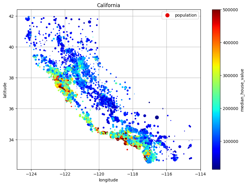
plt.show()We can include more information:
# Include option `s` for population and color for price!
explore.plot(
    kind="scatter",
    title="California",
    x="longitude",
    y="latitude",
    s=explore["population"] / 100,
    label="population",
    c="median_house_value",
    cmap="jet",
    colorbar=True,
    legend=True,
    sharex=False,
    figsize=(10,7),
    grid=True,
    # alpha=0.2,
)
plt.show()
You will see that housing prices are very related to location. A clustering algorithm should be useful for detecting main cluster and for adding new features that measure proximity to the cluster centers. Also, ocean proximity also appears useful but not really up north, so it would be a complicated policy to include.
p. 63
Since the dataset is not huge, let’s compute the standard correlation coefficient (AKA Pearson’s ) between every pair of attributes.
# corr_matrix = explore.corr()
corr_matrix = explore.drop("ocean_proximity", axis=1).corr()
corr_matrix
Cannot compare not numerical values, hence dropping the proximity. There are nicer visuals.
attributes = explore.drop("ocean_proximity", axis=1).columns
pd.plotting.scatter_matrix(explore[attributes], figsize=(12, 8))
plt.show()
We can “zoom in” on a particular graph like this:
explore.plot(
    kind="scatter",
    x="median_income",
    y="median_house_value",
    alpha=0.1,
    grid=True,
)
plt.show()
You can see the horizontal line at the cap, but also some other horizontal lines forming for unknown reasons.
Note, correlation coefficient only measures linear correlations. It can miss nonlinear relationships.
Sometimes, skewed data is better transformed with logarithm or square roots.
The scatter of total bedrooms and members of house hold is very correlated. The book creates some ratios of data.
# Some variables are correlated
explore["rooms_per_house"] = explore["total_rooms"] / explore["households"]
explore["bedrooms_ratio"] = explore["total_bedrooms"] / explore["total_rooms"]
explore["people_per_house"] = explore.population / explore.households

corr_matrix = explore.drop("ocean_proximity", axis=1).corr()
corr_matrix.median_house_value.sort_values(ascending=False)
We look at the correlation to the target value to discover new features. Total rooms has a 13% correlation, and total bedrooms only has a 5% correlation. But the bedroom ratio has a -25% correlation. And rooms per household gives more information than total number of rooms in a district.
Don’t need to be super thorough, just gaining insights into your data. Remember, this is an iterative process.
p. 67
We will write functions for preparing data because:
First, revert to a clean training set by copying again and separate the predictors and labels:
housing = strat_train_set.drop("median_house_value", axis=1) # if not inplace, it return a dataframe
housing_labels = strat_train_set["median_house_value"].copy()
housing.head(3)Most ML algorithms cannot work with missing features and total_bedrooms is incomplete. W have 3 options:
Pandas has a ways to do each thing:
# housing.dropna(subset=["total_bedrooms"], inplace=True)
# housing.drop("total_bedrooms", axis=1)

median = housing.total_bedrooms.median()
housing.total_bedrooms.fillna(median, inplace=True)
But scikit-learn does it better. There’s a sklearn.impute.SimpleImputer class that can store median values for each feature, making it possible to impute missing values for training, test, and validation sets. However, the median can only be computed on numerical attributes, so you need to create a copy of data with only numerical attributes.
from sklearn.impute import SimpleImputer

imputer = SimpleImputer(strategy="median")
housing_num = housing.select_dtypes(include=[np.number]) # only numerical types
imputer.fit(housing_num) # fit imputer on training data
print(imputer.statistics_)  # stores medians here
print(housing_num.median().values)

# replace missing values with _trained_ medians
X = imputer.transform(housing_num)
Other strategies are: mean, most_frequent. You can also specify (stragegy="constant", fill_value="foo"). These last two support non-numerical data.
sklearn.impute package also more powerful imputers like KNNImputer and IterativeImputer. These predict values based on other features in the dataset.
We need to talk about sklearn if we are using it:
fit() method and takes in a dataset as a parameter, labels if applicable, and relative hyperparameters based on the model.transform() method with the dataset to transform as a parameter and it returns the transformed dataset. They also have a fit_transform() method which is like fit() and then transform().predict() method that takes in a dataset of new instances and returns a dataset of corresponding predictions. Also has a score() method to measure quality of predictions.X = imputer.transform(housing_num)
housing_tr = pd.DataFrame(X, columns=housing_num.columns, index=housing_num.index)
housing_tr.head(3)The transform method returns Numpy arrays, which we easily convert back into a data frame.
We only have one text attribute, ocean_proximity. Let’s check it out.
# Return index and column with this format
housing_cat = housing[["ocean_proximity"]] # meow
housing_cat.head(5)
These are actually categories like “NEAR OCEAN” or “INLAND”. We basically perform a technique called one-hot-encoding which creates as many new columns as there are categories and then assigns a 1 or 0 based on if that record has that category.
from sklearn.preprocessing import OrdinalEncoder, OneHotEncoder

ordinal_encoder = OrdinalEncoder()
housing_cat_encoded = ordinal_encoder.fit_transform(housing_cat)
print(ordinal_encoder.categories_) # gives list of categorical attributes

cat_encoder = OneHotEncoder()
housing_cat_1hot = cat_encoder.fit_transform(housing_cat).toarray()
print(cat_encoder.categories_)
We create categories with OrdinalEncoder, which works on its own kind of if the categories are hierarchical, like bad, good, great. But when that is not the case, we one-hot encode.
One issue is that the OneHotEncoder returns a SciPy sparse matrix, instead of a NumPy array. This is a mostly zero matrix. There are so many zeros that under the hood, it only stores nonzero values and their position. But, we need to convert it to an array with .toarray().
Apparently, you can also set OrdinalEncoder(sparse=False)… not sure about that.
Alternatively, pandas has a pd.get_dummies() method but the OneHotEncoder can remember which categories it was trained on, important for for production. This means, given new information, if not all categories are in the dataset, .get_dummies() won’t provide 0 values for missing categories, it will just not know they even existed.
Note that if there are a lot of categories, this methodology could seriously impair training performance. In these cases, could be helpful to look for better features, maybe even a measurement if possible. With neural networks, you might replace each category with a learnable, low-dimensional vector called an embedding. That is for later though.
Feature Scaling is probably one of the most important transformations. Two common ways are min-max scaling and standardization.
Important: Only fit scalers to the training data! Never use .fit() or .fit_transform() on anything other than training sets. Once you have a trained scaler, you can use it to transform() another set, including test and validation sets. The training set will also be scaled to a specified range. If new data contains outliers, they may end up outside the range. You can avoid this by setting clip=True in the hyperparameters.
Min-max (AKA normalization) is simpler. Scikit-learn provides a transformer called MinMaxScaler. You can also change the default range with the featrue_range=(-1,1) hyperparameter if you need to for some reason. Like, neural networks work better with a zero-mean input, so perhaps (-1,1) is preferable there.
from sklearn.preprocessing import MinMaxScaler

min_max_scalar = MinMaxScaler(feature_range=(-1,1))
housing_num_min_max_scaled = min_max_scalar.fit_transform(housing_num)
print(housing_num_min_max_scaled)
MinMaxScalar.fit_transform() returns an array.
Standardization is different, it standardizes value to have a zero mean. It won’t restrict you to a range and is less affected by outliers (and mistakes).
from sklearn.preprocessing import StandardScaler

std_scalar = StandardScaler()
housing_num_std_scaled = std_scalar.fit_transform(housing_num)
print(housing_num_std_scaled)
You can scale a sparse matrix before condensing it by setting StandardScaler(with_mean=False). That only divides by standard deviation without subtracting mean.
Oops, ML models don’t like data with heaby tails. Before scaling, we should try to make distributions symmetrical.
Replacing feature with logarithm can help reduce heavy tails. You can bucketizing the feature too, chop feature into roughly equal-sized buckets, and replace the feature value with the index of the bucket.
Some features, like our median housing age, is multimodal distribution, it has multiple peaks or modes. It can be helpful to bucketize them but then treat the IDs as categories, rather than values. Then you one-hot encode so the model can more easily find patterns. Obviously, you want as few buckets as possible.
You can also transform multimodal distributions to add a feature for each main mode. Typically computed using a radial basis function (RBF), a function that depends on the distance between an input and a fixed point. Common RBF is the Gaussian RBF.
Scikit-Learn has an rbf_kernel() function.
from sklearn.metrics.pairwise import rbf_kernel

age_simil_35 = rbf_kernel(housing[["housing_median_age"]],[[35]], gamma=0.1)
There’s also the case that the target value may need to be transformed. But then the model predicts something like the log of the median house value. Luckily, most of Scikit-learn’s transformers have an inverse_transform() method.
from sklearn.linear_model import LinearRegression

target_scalar = StandardScaler()
scaled_labels = target_scalar.fit_transform(housing_labels.to_frame())

model = LinearRegression()
model.fit(housing[["median_income"]], scaled_labels) # simple regression?
some_new_data = strat_test_set[["median_income"]].iloc[:5].copy() # pretend it is new data

scaled_predictions = model.predict(some_new_data)

# Showing how we can inverse transform our model
predictions = target_scalar.inverse_transform(scaled_predictions)
predictions
But don’t waste your time doing that. Scikit-Learn has a TransformedTargetRegressor class!
# -- OR --
from sklearn.compose import TransformedTargetRegressor

model = TransformedTargetRegressor(
    LinearRegression(),
    transformer=StandardScaler(),
)

model.fit(housing[["median_income"]], housing_labels)
predictions = model.predict(some_new_data)
predictions
Methods are slightly different. The former returns a list of lists, each inner list is just 1 element prediction. The latter just returns a list of predictions.
p. 79
Sometimes, you got to write your own custom transformers. If the transformations do not require training, you can write a function that takes in a NumPy array as input and outputs a transformed array.
Transform heavy tailed distributions with logarithms.
# Custom Transforms
from sklearn.preprocessing import FunctionTransformer

# provide both forwards and backwards functions
log_transformer = FunctionTransformer(np.log, inverse_func=np.exp)
log_pop = log_transformer.transform(housing[["population"]])
The transformation function can also accept hyperparameters as additional arguments.
rbf_tranformer = FunctionTransformer(
    rbf_kernel,
    kw_args=dict(Y=[[35.]], gamma=0.1)
)
age_simil_35 = rbf_tranformer.transform(housing[["housing_median_age"]])
age_simil_35
You can include multiple values, as shown in the book. You can also just use a lambda function, to find or something like that.
What if we need the transformer to be trainable, to learn some parameters in the fit() method and use them later in the transform() method. You need a custom class, which is why Scikit-Learn relies on duck typing.
# Custom tranformer to act like StandardScaler
from sklearn.base import BaseEstimator, TransformerMixin
from sklearn.utils.validation import check_array, check_is_fitted

class StandardScalerClone(BaseEstimator, TransformerMixin):
    def __init__(self, with_mean=True):
        self.with_mean = with_mean

    def fit(self, X, y=None):
        X = check_array(X)
        self.mean_ = X.mean(axis=0)
        self.scale_ = X.std(axis=0)
        self.n_features_in_ = X.shape[1]
        return self

    def transform(self, X):
        check_is_fitted(self)
        X = check_array(X)
        assert self.n_features_in_ == X.shape[1]
        if self.with_mean:
            X = X - self.mean_
        return X / self.scale_
The TransformerMixin gives you fit_transform() for free. The BaseEstimator give you get_params() and set_params().
Production code should check inputs, but development code is ok if we don’t from now on. The fit() method needs all params and must return self. All estimators should also set feature_names_in_ in the fit() method. The book includes an example whose fit() method uses the sklearn.cluster.KMeans class… Oh I guess we need it…
from sklearn.cluster import KMeans

class ClusterSimilarity(BaseEstimator, TransformerMixin):
    def __init__(self, n_clusters=10, gamma=1.0, random_state=None) -> None:
        self.n_clusters = n_clusters
        self.gamma = gamma
        self.random_state = random_state

    def fit(self, X, y=None, sample_weight=None):
        self.kmeans_ = KMeans(self.n_clusters, random_state=self.random_state)
        self.kmeans_.fit(X, sample_weight=sample_weight)
        return self

    def tranform(self, X):
        return rbf_kernel(
            X,
            self.kmeans_.cluster_centers_,
            gamma=self.gamma,
        )

    def get_feature_names_out(self, names=None):
        return [
            f"Cluster {i} similarity" for i in range(self.n_clusters)
        ]
After training, the cluster centres are available via the cluster_centers_ attribute.
cluster_simil = ClusterSimilarity(n_clusters=10, gamma=1., random_state=42)
similarities = cluster_simil.fit_transform(
    housing[['latitude', 'longitude']],
    sample_weight=housing_labels
)
similarities
This uses k-means to locate clusters and measure Gaussian RBF similarity between each district and all 10 (default) cluster centers.
The Pipeline class helps perform a sequence of transformation in the right order.
from sklearn.pipeline import Pipeline

num_pipline = Pipeline([
    ("impute", SimpleImputer(strategy="median")),
    ("stanardize", StandardScaler()),
])
Those are your steps in tuples of name and class. Names can be anything unique without a dunder-score (__). Estimators must all be transformers, needing the .fit_transform() method, except the last one, which can be anything!
Note: In jupyter notebook, you can import sklearn and then sklearn.set_config(diaplay="diagram"). Estimators will render as interactive diagrams.
You can also use the sklearn.pipeline.make_pipeline() function if you don’t want to name your steps, just pass in your transformers in order.
When you call the pipeline’s fit() method, it calls fit_transform() sequentially on all transformers. The pipeline exposes all same methods as the final estimator. Give it a go:
from sklearn.pipeline import Pipeline

num_pipline = Pipeline([
    ("impute", SimpleImputer(strategy="median")),
    ("stanardize", StandardScaler()),
])

housing_num_prepared = num_pipline.fit_transform(housing_num)
housing_num_prepared[:3].round(3)
Now, we want a Data Frame I think
df_housing_num_prepared = pd.DataFrame(
    housing_num_prepared,
    columns=num_pipline.get_feature_names_out(),
    index=housing_num.index,
)
df_housing_num_prepared.head(5)
Pipelines support indexing! You can also access your named pipeline estimators like num_pipeline["simpleimputer"] if needed.
Ok, so we have been handeling categorical and numerical columns separately, but want a single transformer for all columns. Hello sklearn.compose.ColumnTransformer.
# One Transformer to rule them all
from sklearn.compose import ColumnTransformer
from sklearn.pipeline import make_pipeline


all_cols = housing.columns
cat_attribs = ["ocean_proximity"]
num_attribs = [x for x in all_cols if x not in cat_attribs]
# print(num_attribs)

cat_pipeline = make_pipeline(
    SimpleImputer(strategy="most_frequent"),
    OneHotEncoder(handle_unknown="ignore"),
)

preprocessing = ColumnTransformer([
    ('num', num_pipline, num_attribs),
    ('cat', cat_pipeline, cat_attribs),
])
The ColumnTransformer takes a list of triple tuples because we need to specify the affected columns in each transformation.
Instead of a transformer you may also pass "drop" to drop a column, or "passthrough" to leave it be. By default, remaining columns (not listed) are dropped. You can set remainder hyperparameter to "passthrough" or any transformer to handle differently.
FFS…
# One Transformer to rule them all
from sklearn.compose import make_column_selector, make_column_transformer

preprocessing = make_column_transformer(
    (num_pipline, make_column_selector(dtype_include=np.number)),
    (cat_pipeline, make_column_selector(dtype_include=object)),
)
Multiple ways to do everything.
And finally…
housing_prepared = preprocessing.fit_transform(housing)This pre-processing pipeline takes the entire training dataset and applies each transformer to the appropriate column. Then it concatenates the transformed columns horizontally and returns a NumPy array. So get column names with preprocessing.get_feature_names_out().
What transformation have we made and why?
Here you go:
# Build pipeline altogether now!
def column_ratio(X):
    return X[:,[0]] / X[:,[1]]

def ratio_name(function_transformer, feature_names_in):
    return ["ratio"]

def ratio_pipeline():
    return make_pipeline(
        SimpleImputer(strategy="median"),
        FunctionTransformer(column_ratio, feature_names_out=ratio_name),
        StandardScaler(),
    )

log_pipline = make_pipeline(
    SimpleImputer(strategy="median"),
    FunctionTransformer(np.log, feature_names_out="one-to-one"),
    StandardScaler(),
)

cluster_simil = ClusterSimilarity(n_clusters=10, gamma=1.0, random_state=42)
default_num_pipeline = make_pipeline(
    SimpleImputer(strategy="median"),
    StandardScaler(),
)

preprocessing = ColumnTransformer(
    [
        ("bedrooms", ratio_pipeline(), ["total_bedrooms", "total_rooms"]),
        ("rooms_per_house", ratio_pipeline(), ["total_rooms", "households"]),
        ("people_per_house", ratio_pipeline(), ["population", "households"]),
        ("log", log_pipline, ["total_bedrooms", "total_rooms", "population", "households", "median_income"]),
        ("geo", cluster_simil, ["latitude", "longitude"]),
        ("cat", cat_pipeline, make_column_selector(dtype_include=object)),
    ],
    remainder=default_num_pipeline,
)

housing_prepared = preprocessing.fit_transform(housing)
print(housing_prepared.shape)
print(preprocessing.get_feature_names_out())The hard work is mostly over. Let’s make a simple linear regression model.
from sklearn.linear_model import LinearRegression

lin_reg = make_pipeline(preprocessing, LinearRegression())
lin_reg.fit(housing, housing_labels)

housing_predictions = lin_reg.predict(housing)
print(housing_predictions[:5].round(-2))
print(housing_labels.iloc[:5].values)
We want to use the RMSE as the performance measure, so lets measure the entire training set.
from sklearn.metrics import mean_squared_error
lin_rmse = mean_squared_error(
    housing_labels,
    housing_predictions,
    squared=False
)
lin_rmse
The current typical predictions error is about $68,648… not great. This is an example of underfitting, our model has not learned enough. The features do not provide enough information to make good predictions, or the model is not powerful enough.
The model is not regularized, so we reduce constraints. Lets try a better model. How about the DecisionTreeRegresso. More on this later in the book, just a quick introduction now.
from sklearn.tree import DecisionTreeRegressor

tree_reg = make_pipeline(
    preprocessing,
    DecisionTreeRegressor(random_state=42),
)

# Training in progress
tree_reg.fit(housing, housing_labels)
That gave me a strange graphical output… Anyway
# Look at results against training data
housing_predictions = tree_reg.predict(housing)
tree_rmse = mean_squared_error(
    housing_labels,
    housing_predictions,
    squared=False
)
tree_rmse
The error is . This is a sure sign of overfitting.
p. 89
We could split the training set into smaller sets with validation sets as well, and train on those… But Scikit-Learn has that covered. The cross_val_score() randomly splits the training set into 10 non-overlapping subsets called folds. It trains and evaluates the decision tree model 10 times, picking a different fold evaluation each time and using the other 9 for training.
from sklearn.model_selection import cross_val_score

tree_rmses = -cross_val_score(
    tree_reg, housing, housing_labels, scoring="neg_root_mean_squared_error", cv=10,
)
pd.Series(tree_rmses).describe()
This model performs just as bad seemingly.
We will look at RandomForestRegressor another one in a later chapter. It works by training many decision trees on random subsets of features, and then averaging out predictions. A model composed of many other models is called an ensemble.
This one takes a bit longer to run.
from sklearn.ensemble import RandomForestRegressor

forest_reg = make_pipeline(
    preprocessing,
    RandomForestRegressor(random_state=42),
)
forest_rmses = -cross_val_score(
    forest_reg, housing, housing_labels, scoring="neg_root_mean_squared_error", cv=10
)
pd.Series(forest_rmses).describe()
It does a lot better, but if you train on the entire set, you will see some overfitting again. Possible solutions:
Finally, just going to try on my own, the Multi-Layer Perceptron Regressor. I think it is working…
from sklearn.neural_network import MLPRegressor

mlp_regressor = make_pipeline(
    preprocessing,
    MLPRegressor(),
)
mlp_rmses = -cross_val_score(
    mlp_regressor, housing, housing_labels, scoring="neg_root_mean_squared_error", cv=5
)
pd.Series(mlp_rmses).describe()
I changed the cross validation to 5 and one round is taking nearly 2 minutes to complete. Took nearly 10 minutes for a mean of 164,613 error…
If you have a short list of models, you can fine-tune them.
You can fiddle with hyperparameter manually or use GridSearchCV. It uses cross-validation to evaluate all possible combinations of hyperparameter values.
from sklearn.model_selection import GridSearchCV

full_pipeline = Pipeline(
    [
        ("preprocessing", preprocessing),
        ("random_forest", RandomForestRegressor(random_state=42)),
    ]
)
param_grid = [
    {
        'preprocessing__geo__n_clusters': [5,8,10],
        'random_forest__max_features': [4,6,8],
    },
    {
        'preprocessing__geo__n_clusters': [10,15],
        'random_forest__max_features': [6,8,10],
    },
]
grid_search = GridSearchCV(
    full_pipeline, param_grid, cv=3, scoring='neg_root_mean_squared_error',
)
grid_search.fit(housing, housing_labels)
You can refer to any hyperparameter of any estimator in a pipeline. For preprocessing__geo__n_clusters it splits at the dunder-scores:
preprocessing, finding the ColumnTransformer.ClusterSimilarity transformer we named "geo"n_clusters hyperparameter and tunes it.Wrapping preprocessing steps in a pipeline allows you to tune the preprocessing hyperparameters along with the model hyperparameters. If fitting the pipeline transformer is computationally expensive, you can set the pipeline’s memory parameter to the path of a caching directory. It saves the transformer with those parameters there to load if called again.
Looking at the code, param_grid instructs models to be trained But the grid_search also uses cv=3 making it 45 models. It took almost 10 minutes for me.
print(grid_search.best_estimator_) # only used RandomForestRegressor
grid_search.best_params_
The best model is obtained when n_clusters=15 and max_features=6.
If GridSearchCV is initialized with refit=True (which is default), once it finds the best estimators with cross-validation, it retrains it on the whole training set.
cv_res = pd.DataFrame(grid_search.cv_results_)
cv_res.sort_values(by="mean_test_score", ascending=False, inplace=True)
cv_res.rename(
    {
        "param_preprocessing__geo__n_clusters": "n_clusters",
        "param_random_forest__max_features": "max_features",
    },
    inplace=True,
    axis='columns',
)
cv_res.head()
Since the n_clusters is at 15, our max, you could go higher to see is possibly more makes it better.
I did this with max of 20 and the selection is better at 20… Let’s move forward.
GridSearchCV will run all combinations, which is the best option, but only realistic if you don’t have too many combinations. Another idea is trying only a random selection of hyperparameters. It’s continuous nature can make testing more robust and random selection makes it run faster.
from sklearn.model_selection import RandomizedSearchCV
from scipy.stats import randint

param_distribs = {
    'preprocessing__geo__n_clusters': randint(low=5, high=7),
    'random_forest__max_features': randint(low=20, high=50),
}

rnd_search = RandomizedSearchCV(
    full_pipeline,
    param_distributions=param_distribs,
    n_iter=10,
    cv=3,
    scoring="neg_root_mean_squared_error",
    random_state=42,
)

rnd_search.fit(housing, housing_labels)
I like it. There are also HalvingRandomSearchCV and HalvingGridSearchCV hyperparameter search classes in Scikit-Learn. Their goals is to use resources more efficiently. It uses limited resources first, small part of training set. Only best candidates are selected for additional training and evaluation. This continues to tune hyperparameters.
Random Search found best params of n_clusters=6 and max_features=40
You can gain insights by inspecting the best model. The RandomForestRegressor lets you view importance of features.
final_model = rnd_search.best_estimator_
feature_importances = final_model["random_forest"].feature_importances_
sorted(
    zip(
        feature_importances,
        final_model['preprocessing'].get_feature_names_out(),
    ),
    reverse=True
)
You can see that a lot of the ocean_proximity features are pretty useless.
Scikit-Learn has a sklearn.feature_selection.SelectFromModel transformer that can automatically drop the lest useful features.
You can try to understand other errors and fix issues by:
p. 96
X_test = strat_test_set.drop("median_house_value", axis=1)
y_test = strat_test_set.median_house_value.copy()

final_predictions = final_model.predict(X_test)

final_rmse = mean_squared_error(y_test, final_predictions, squared=False)
print(final_rmse)
You can also get a 95% confidence interval with
from scipy import stats
confidence = 0.95
squared_errors = (final_predictions - y_test)**2
np.sqrt(
    stats.t.interval(
        confidence,
        len(squared_errors)-1,
        loc=squared_errors.mean(),
        scale=stats.sem(squared_errors),
    )
)
At this point, do not tweak any hyperparameter to make the validation look better, that will begin to overfit.
import joblib

joblib.dump(final_model, "my_california_housing_model.pkl")
To use the model, you will need the same imports pretty much that the model was built with. Then you use joblib.load('file.pkl') to bring in the model.
You can wrap your model in a dedicated web service that your web application can query through a REST API. Then you can build your application in any language to use your API.
You can deploy your pickle to Google’s Vertex AI Cloud. It handles load balancing and scaling for you and act like a JSON API.
From here you need to write monitoring code to check the system’s live performance at regular intervals. You should have alerts for when performance drops.
If data keeps evolving, you must keep updating the datasets and retraining your model. Here’s what you can automate:
Also evaluate the model’s input data quality. Failing sensor and other data inputs can be and issue.
Keep a backup of all models you create and be able to rollback a model quickly if it fails badly for some reason.
p. 103 - 130
The MNIST dataset is a set of 70,000 small images of handwritten digits by people. This set is basically the “Hello, world!” of machine learning. In fact, Scikit-Learn helps you download the set.
from sklearn.datasets import fetch_openml

mnist = fetch_openml('mnist_784', as_frame=False, parser='auto')
Scikit-Learn has fetch_*, load_*, and make_* functions that pull from the internet, pull from disk, and create dataset.
Our type(mnist) dataset is a sklearn.utils._bunch.Bunch object. Using print(dir(mnist)) we has a DESCR for description, data, categories, target, etc… We set the as_frame=False because there are images and a DataFrame isn’t designed for that. images are and each number represents pixel intensity from 0 to 255.
We need to grab an instance’s feature vector, reshape it to array, and display it with Matplotlib’s imshow() function.
import matplotlib.pyplot as plt

def plot_digit(image_data):
    """
    Takes in an array of pixels, reshapes into 28x28 and displays as a b&w image

    Args:
        image_data (np.array): an array of pixels to be transformed
    """
    image = image_data.reshape(28,28)
    plt.imshow(image, cmap='binary')
    plt.axis('off')

plot_digit(X[0])
plt.show()
print(y[0])
plot_digit(X[5])
plt.show()
print(y[5])
If you don’t include cmap='binary', it tries to produce a colourful image, which is purple background and yellow drawing, pretty cool, but not correct. The binary setting makes it black and white.
This dataset is already split into train and test. The first 60k are training and the last 10k are test. This is helpful for consistency. Also, some learning algorithms are sensitive to the order of training instances and perform poorly if they coincidently get similar instances in a row.
Let’s simplify and try to identify just one digit, 5. This is a Boolean, binary classifier, capable of distinguishing between 2 classes, “5” and “not-five”. We transform labels into binary
y_train_5 = (y_train == '5')
y_test_5 = (y_test == '5')
And then use stochastic gradient descent (SGD) classifier, sklearn.linear_model.SGDClassifier. It is good at handling large datasets efficiently because it trains instances independently. Good for online learning as well.
from sklearn.linear_model import SGDClassifier

sgd_clf = SGDClassifier(random_state=42)
sgd_clf.fit(X_train, y_train_5)
It’s easy to type but takes a while to train… 36s for my computer.
This, sgd_clf.predict(X[0]) gives error because it is an array of digits. It expects it to be in a list:
sgd_clf.predict([X[0]])The error also suggests reshaping the array.
There are many performance measures available. However, evaluating a classifier is more difficult than a regressor.
We will start with using the sklearn.model_selection.cross_val_score to evaluate our classifier.
from sklearn.model_selection import cross_val_score

cross_val_score(
    sgd_clf, # predictor
    X_train, # training data
    y_train_5, # training labels
    cv=3,
    scoring='accuracy'
)
Impressive 95%, but is that right?
from sklearn.dummy import DummyClassifier

dummy_clf = DummyClassifier()
dummy_clf.fit(X_train, y_train_5)
cross_val_score(
    dummy_clf, # predictor
    X_train, # training data
    y_train_5, # training labels
    cv=3,
    scoring='accuracy'
)
Apparently the DummyClassifier just labels with the most common value. In our case, it is False, meaning it is 90% accurate.
Accuracy is not a preferred performance measure for classifiers, especially with skewed datasets. Skewed datasets probably aren’t great either.
A better way to evaluate is with a confusion matrix (CM).
The book on p. 108 shows how to create your own cross validation function using sklearn.model_selection.StratifiedKFold.
p. 108
Confusion matrix counts number of times instances of A are classified as B.
To avoid touching the test set we will use sklearn.model_selection.cross_val_predict which is just like it’s brother only it returns the predictions instead of evaluation scores. You get clean predictions, out-of-sample, predictions on data the model never saw during training.
from sklearn.model_selection import cross_val_predict

y_train_5_pred = cross_val_predict(
    sgd_clf,
    X_train,
    y_train_5,
    cv=3
)
Now, use sklearn.metrics.confusion_matrix
from sklearn.metrics import confusion_matrix

cm = confusion_matrix(y_train_5, y_train_5_pred)
cm
it will be like
| na | Pred. False | Pred. True |
|---|---|---|
| Act. False | 53,892 | 687 |
| Act. True | 1,891 | 3,530 |
It missed 1,891 and incorrectly labelled 687. Maybe you remember this from your Data Science course:
Where is true positive. Precision is about 83.7%, but itself can be miss leading. It can incorrectly label many as False and still have 100% precision if what it labelled True was correct.
Because of the larger number of false negatives recall is about 65.1%.
Don’t believe me?
from sklearn.metrics import precision_score, recall_score, f1_score

print(precision_score(y_train_5, y_train_5_pred))
print(recall_score(y_train_5, y_train_5_pred))
print(f1_score(y_train_5, y_train_5_pred))
What is score? It is a harmonic mean of precision and recall, which gives more weight to low values. So it only get a high score if both values are high.
The precision/recall trade-off means that as you increase precision you reduce recall, and vice versa.
The book looks at how SGDClassifier makes classifications. In terms of the confusion matrix, values can be shifted left to right or right to left, but they move by column, not by cell.
The SGDClassifier has a decision_function([some_digit]) that compares an images score to a threshold. You cannot access the threshold directly, but you can play with that function.
from sklearn.metrics import precision_recall_curve
# investigate threshold

y_scores = cross_val_predict(
    sgd_clf,
    X_train,
    y_train_5,
    cv=3,
    method='decision_function'
)

precisions, recalls, thresholds = precision_recall_curve(y_train_5, y_scores)

plt.plot(thresholds, precisions[:-1], 'b--', label='Precision', linewidth=2)
plt.plot(thresholds, recalls[:-1], 'g-', label='Recall', linewidth=2)
# plt.vlines(thresholds, 0, 1.0, 'k', 'dotted', label='threshold')
plt.legend()
plt.grid(linewidth=2)
plt.show()
Interesting curve. You can also just plot recall against precision
plt.plot(recalls, precisions, linewidth=2, label='precision/recall curve')
plt.ylabel('Precision')
plt.xlabel('Recall')
plt.hlines(0.9, 0, 1.0, 'k', 'dotted', label='threshold')
plt.grid(linewidth=2)
plt.legend()
plt.show()
That is a line at precision at 90%, crosses recall just above 40%.
# Pretend predictions with Precision at 90%
idx_for_90_precision = (precisions >= 0.90).argmax() # index of largest
threshold_for_90_precision = thresholds[idx_for_90_precision]
print(threshold_for_90_precision)

# making predictions
y_train_pred_90 = (y_scores >= threshold_for_90_precision)
print(precision_score(y_train_5, y_train_pred_90))
print(recall_score(y_train_5, y_train_pred_90))
You’ll see that precision is just at 90%, but recall drops to 48.0%.
The Receiver Operating Characteristic (ROC) curve is another common tool for binary classifiers. It plots true positive rate (recall) against false positive rate (fall-out).
It is where the true negative rate is called specificity.
from sklearn.metrics import roc_curve

fpr, tpr, thresholds = roc_curve(y_train_5, y_scores)
indx_for_threshold_at_90 = (thresholds <= threshold_for_90_precision).argmax()
tpr_90, fpr_90 = tpr[indx_for_threshold_at_90], fpr[indx_for_threshold_at_90]

plt.plot(fpr, tpr, linewidth=2, label='ROC Curve')
plt.plot([0,1], [0,1], 'k:', label="Random classifier's ROCS Curve")
plt.ylabel('Recall: True Positive')
plt.xlabel('Fall-out: False Positive')
plt.grid(linewidth=2)
plt.legend()
plt.show()
We can compare classifiers by measuring the area under the curve (AUC). Perfect classifier has ROC AUC of 1.
from sklearn.metrics import roc_auc_score
roc_auc_score(y_train_5, y_scores)
Rule of thumb is to prefer the Precision/Recall (PR) curve to the ROC Curve when the positive class is rare. I mean, judging by the 96% score from above, this classifier looks nice again.
The sklearn.ensemble.RandomForestClassifier does not have a decision_function, but a predict_proba() method to return class probabilities for each instance. So, it returns probabilities regarding what it thinks is the answer, really cool!
from sklearn.ensemble import RandomForestClassifier

forest_clf = RandomForestClassifier(random_state=42)
y_probas_forest = cross_val_predict(
    forest_clf,
    X_train,
    y_train_5,
    cv=3,
    method="predict_proba"
)
y_probas_forest[:2]
The model can appear overconfident. Look into the sklearn.calibration package to make estimated probabilities closer to actual probabilities.
The book also plots a precision recall curve… The curve is similar to before but the AUC is a bit closer to 1.
y_train_pred_forest = y_probas_forest[:,1] >= 0.5 # Probability >= 50%
f1_score(y_train_5, y_train_pred_forest)
You have to extract predictions more manually apparently.
p. 119
We will move now to muliclass, or multinomial, classifiers. Scikit-Learn’s SGDClassifier and SVC classes are strictly binary classifiers. However, the LogisticRegression, RandomForestClassifier, and GaussianNB can handle multiple classes.
There are ways to use binary, like a One-Versus-All (OVA), or one-versus-the-rest method where you train binary classifiers against all classes, so for each digit in our case, and you compare the digit scores from each classifier for an image.
Alternatively, you can train a binary classifier for every pair of digits. This is a One-versus-One strategy. you would require classifiers, 45 in our case. Algorithms, like SVG, scale poorly with data and so an OvO strategy is preferred because it is quick to train many smaller classifiers. However, OvR is preferred for most other binary classification algorithms.
With that bit of knowledge, Scikit-Learn can detect when it needs to employ OvR or OvO, making binary classifiers appear multinomial. Let’s try!
# Employing OvO
from sklearn.svm import SVC

svm_clf = SVC(random_state=42)
svm_clf.fit(X_train[:2000], y_train[:2000])

svm_clf.predict([X[0]])
There are regular classes OneVsOneClassifier and OneVsRestClassifier.
from sklearn.multiclass import OneVsRestClassifier

ovr_clf = OneVsRestClassifier(SVC(random_state=42))
ovr_clf.fit(X_train[:2000], y_train[:2000])
ovr_clf.predict([X[0]])
We can also use the SGDClassifier again, stochastic gradient descent, which uses a OvR strategy under the hood.
sgd_clf = SGDClassifier(random_state=42)
sgd_clf.fit(X_train, y_train)
sgd_clf.predict([X[0]])
This one is not quick nor correct. Took over 4m. You can sgd_clf.decision_function([X[0]]).round() to see a lot of scores look similar.
cross_val_score(sgd_clf, X_train, y_train, cv=3, scoring='accuracy')Try cross validation to see it gets roughly 86% accuracy, which isn’t too bad. A DummyClassifier would only get 10% because we have 10 classes now.
We can scale inputs to improve accuracy.
from sklearn.preprocessing import StandardScaler

scaler = StandardScaler()
X_train_scaled = scaler.fit_transform(X_train.astype("float64"))
print(X_train_scaled[:10])
cross_val_score(sgd_clf, X_train_scaled, y_train, cv=3, scoring="accuracy")
I think it is a little weird to scale pixel data, but never the less necessary! Accuracy improves slightly.
p. 122
For a real project, we can revert back to the steps on the machine learning project checklist. You’d explore multiple models and fine-tune hyperparameters using GridSearchCV.
Assume we have our model and we want to improve it. We can analyse the types of errors it makes. We want to look at a confusion matrix again, but we will use the sklearn.metrics.ConfusionMatrixDisplay class instead of the function for better visuals.
# Let's look at a confusion matrix!

from sklearn.metrics import ConfusionMatrixDisplay

# Makes predictions for all values, trained on slightly different models
y_train_pred = cross_val_predict(sgd_clf, X_train_scaled, y_train, cv=3)
ConfusionMatrixDisplay.from_predictions(y_train, y_train_pred)
plt.show()
One thing we can note… whenever it’s done running… “5” has less correct guesses. It’s important to normalize to see if that is because it was actually wrong, or if there were just less 5’s to guess right. Normalizing is easy, after it loads…
ConfusionMatrixDisplay.from_predictions(
	y_train, y_train_pred, normalize='true', values_format='.0%'
)
plt.show()
You can see that the model guessed 5 was 5 correctly 82% of the time, and predicted 5 was 8 10% of the time.
We can change how it looks by putting zero weight on the correct predictions.
# 0-weight on correct predictions
sample_weight = (y_train_pred != y_train)
ConfusionMatrixDisplay.from_predictions(
    y_train, y_train_pred, sample_weight=sample_weight, normalize='true', values_format='.0%'
)
plt.show()
That shows clearly that many incorrect guesses think the value is an 8 when it isn’t. Interpretation is key. 65% or misclassified 0s were incorrectly classified as 8s. But only 6% or 0s were miss classified, . Changing normalize='pred' normalizes based on column instead of row.
# 0-weight on correct predictions, normalized 'pred'
sample_weight = (y_train_pred != y_train)
ConfusionMatrixDisplay.from_predictions(
    y_train, y_train_pred, sample_weight=sample_weight, normalize='pred', values_format='.0%'
)
plt.show()
You can see that 56% of misclassified 7s are actually 9s. It’s a different way to view errors.
So, we know an error is false 8s. How do we reduce that error? You can gather data or write an algorithm to count “closed loops”, signature of an 8. The latter would be a new feature. We can also preprocess the images with Scikit-Image, Pillow, or OpenCV to make patterns, like closed loops, stand out more.
You can also have a look at individual cases where the error occurs. Somehow the book plots images in a confusion matrix.
The SGDClassifier assigns a weight per class to each pixel. Some numbers are quite similar and so their summed scores would be very close. So, to improve results, we could preprocess to center images and ensure little-to-no rotation.
Better yet, we can introduce shifted and rotated images so the model can better learn and tolerate such variations!
We will cover data augmentation later (Ch. 14).
p. 125
When would you was a model to output multiple classes? Maybe a face-recognition classifier for images of multiple people. A multilabel classification system outputs multiple binary tags given its input.
import numpy as np
from sklearn.neighbors import KNeighborsClassifier

y_train_large = (y_train >= '7')
y_train_odd = (y_train.astype('int8')%2==1)
y_multilabel = np.c_[y_train_large, y_train_odd]

knn_clf = KNeighborsClassifier()
knn_clf.fit(X_train, y_multilabel)
It’s a cool idea, creating multiple labels. The np.c_ concatenates arrays. Also, KNeighborsClassifier supports multilabel classification.
To evaluate a multilabel classifier, you could use the score for each individual label and then average together.
knn_pred = cross_val_pred(knn_clf, X_train, y_multilabel, cv=3)
f1_score(y_multilabel, knn_pred, average='macro')
The f1_score() function has that built in, but assumes labels are equally important. However, if there are more images of small numbers than large, you may want to set average='weighted' which weighs based on instances.
SVC does not natively support multilabel classification. You can train separate models per label, but they wouldn’t capture dependencies between labels. In our case, large numbers are and you can see that odd are twice as likely as even. You can organize models in a chain, where output of one model is fed into the input of another.
Scikit-Learn has a ChainClassifier for this.
from sklearn.multioutput import ClassifierChain

chain_clf = ClassifierChain(SVC(), cv=3, random_state=42)
chain_clf.fit(X_train[:2000], y_multilabel[:2000])
chain_clf.predict([X[0]])p. 127
Multioutput classification is a generalization of multilabel classification where each label can be multiclass (have multiple labels). The book wants to build a system to remove noise from images. So, the classifier output would be multilabel (one label per pixel), and each label can have multiple values (pixel intensity). There is s a hint of regression here in predicting values.
from sklearn.neighbors import KNeighborsClassifier

knn_clf = KNeighborsClassifier()
knn_clf.fit(X_train_loud, y_train_loud)
clean_digit = knn_clf.predict([X_test_loud[0]])
plot_digit(clean_digit)
plt.show()
Training this model was really quick actually. and quite good.
The book recommends continuing training with the KNeighborsClassifier and hyperparameter tuning to achieve over 97% accuracy. Then, add shifted values to the training set. Artificially growing the training set is called data augmentation, or training set expansion.
Another "Hello, world!" dataset is the Titanic dataset (look on Kaggle), or homl.info/titanic with the goal of creating a classifier to predict a Survived column… a bit morbid.
Apache also has an Apache SpamAssassin’s Public Datasets if you want to tackle a spam classifier.
p. 131 - 175
We have used many ML models and training algorithms, but haven’t looked inside of them yet. You can do a lot without knowing implementation details. However, and understanding of this will help you choose an appropriate model, choose the right training algorithm, and choose the best hyperparameters for your task.
Additionally, you will be able to perform error analysis more efficiently and debug issues quickly. And, these topics are essential in understanding, building, and training neural networks.
We are going to dive into a lot of regression.
p. 132
A linear equation is a dependent variable, predicted value, equal to the sum of independent variables multiplied by coefficients, weights, plus a bias term, the y-intercept.
The are feature values, and are model parameters. You can write in vector format as well:
The book doesn’t use vector arrows, but is the feature vector with where always. We also call the hypothesis function.
The above technically gives a scalar value result. We can also use cross product like
You get nearly the same result, but it is a single cell matrix instead of scalar.
We train the model by setting its parameters so that it fits the training data. That is, we find that minimizes the root mean squar error, very common performance measure for regression. It’s actually simpler to minimize the mean square error, and you get the same result.
Note: learning algorithms often optimize a different loss function during training than the performance measure used to evaluate the final model. Many reasons, such as certain functions are easier to optimize and/or have extra terms only needed for training, like for regularization.
The normal equation is a closed-form solution (mathematical equation for direct result) to find the that minimizes the MSE.
Where:
In the code, we use linear algebra baked into Numpy to solve for a fake data we made up. The calculation is close but not exact because of the noise injected via the random uniform function.
from sklearn.preprocessing import add_dummy_feature

x_b = add_dummy_feature(x) # adds x0 = 1 to each instance?
theta_best = np.linalg.inv(x_b.T @ x_b) @ x_b.T @ y
theta_best
We add a dummy feature because remember that is the -intercept so must always be equal to one! If you don’t include it, then you won’t get a prediction for the -intercept.
x_new = np.array([[0],[10]])
x_new_b = add_dummy_feature(x_new)
y_pred = x_new_b @ theta_best
print(y_pred)

plt.scatter(x, y)
plt.plot(x_new, y_pred, "r-", label="Predictions")
plt.ylabel('y')
plt.xlabel('x')
plt.legend()
plt.grid(linewidth=1)
plt.show()
The line looks really close.
Of course, Scikit-Learn has it’s own class for sklearn.linear_model.LinearRegression.
lin_reg = LinearRegression()
lin_reg.fit(x,y)
print(lin_reg.intercept_, lin_reg.coef_)
print(lin_reg.predict(x_new))
Output:
[4.03215906] [[6.93335342]]
[[ 4.03215906]
 [73.36569331]]
This class is based on the scipy.linalg.lstsq() function, named for “least squares”.
The function computes where is the pseudoinverse of . More specifically, the Moore-Penrose inverse. It is computed using a standard matrix factorization technique called singular value decomposition (SVD). It decomposes the training set matrix into the matrix multiplication of 3 other matrices. I think this is beyond the scope of learning, but feel free to look it up.
The Normal equation computes the inverse of , which is matrix, is number of features. The computational complexity can go up to , depending on implementation. That means, more features causes some very rapid growth in complexity. Hence, doesn’t scale well with data.
p. 138
Gradient descent iteratively tweaks parameters to minimize the cost function. To start, you typically fill with random values, called random initialization. Then you make small changes to parameters until the algorithm converges to a minimum error for the cost function.
The step size is very important, determined by the learning rate hyperparameter. If it is too small, then it will take forever to converge. Too high, and you could cause the algorithm to diverge, and completely fail to find a good solution, just circling around the best answer but never landing on it.
Also, not all cost functions are nice, convex continuous functions. In fact, the algorithm could get stuck in a local minimum and miss a global minimum.
Fortunately, the MSE cost function for linear regression model happens to be a convex function. It only has a global minimum and is continuous.
Scaling your variables is also important here. They should be scaled the same so the learning rate applies equally to all of them. Use the StandardScaler class.
To implement gradient descent, you must calculate how much the cost function will change for small changes in . Yes, these are partial derivatives. Partial derivatives of the cost function:
You might remember from the advanced maths notes, the del operator is for partial derivatives in a vector field. You find the Gradient vector like:
This formula involves calculations over the full training set at each gradient step. Because of this, it is really slow with very large training sets. But it scales well with the larger number of features.
Since we know which way is “uphill”, we go the opposite way. Now, we also introduce the learning rate we call (eta).
Gradient decent step:
I tried but am getting overflow error.
# Ad-hoc gradient descent
eta = 0.01 # learning rate
n_epochs = int(1000)
m = int(len(x_b))

theta = np.random.randn(2,1).astype(np.float64) # random init model params

for epoch in range(n_epochs):
    gradients = (x_b @ theta)
    gradients -= y
    gradients = x_b.T.astype(np.float64) @ gradients.astype(np.float64)
    gradients = (2 / m) * gradients
    theta = theta - eta * gradients

theta
Compared to the book, this formula is a mess. I tore it apart only to eventually learn that the learning rate was too high for my formula. Additionally, the epochs are important. It is the number of iterations. If it is too low, you won’t find the optimal parameters. But too high can waste time.
Stochastic gradient descent aims to address the issue of large amounts of training data taking very long to train. It only works on a single instance at a time. This processes much faster but the results are much more volatile as they reach the minimum for the cost function. The final parameters will be quite good, but not optimal.
A learning schedule is a function that determines the learning rate at each iteration. The book gives code on p. 146. When using stochastic gradient descent, the training instances must be independent and identically distributed (IID). You can shuffle the training set at the beginning of each epoch to ensure this.
Lucky for us there is sklearn.linear_model.SGDRegressor!
sgd_reg = SGDRegressor(
    max_iter=1_000,
    tol=1e-5,
    penalty=None,
    eta0=0.01,
    n_iter_no_change=100,
    random_state=69
)
sgd_reg.fit(x, y.ravel()) # y.ravel() because f() expects 1D targets.
print(sgd_reg.intercept_, sgd_reg.coef_)This is a happy medium between batch (full) gradient descent and stochastic gradient descent. It computes gradients on small random sets of instances called mini-batches. You get a good performance boost from hardware optimization of matrix operations, especially when using GPUs.
p. 149